Traffic Flow Simulator

Overview demo

This video is a demonstration of simulating traffic flow within and between intersections/local networks using a tcp/ip server and multiple clients. The clients have factories that either create cars or receive them from the server. The client then simulates the traffic flow until the cars arrive at a "sink" or graph exit. The sink may be a normal sink or a network sink. For a normal sink, the vehicles are simply removed from the graph. If it is a network sink the car data is sent on to the server.

http://www.youtube.com/watch?v=f1qgI55ULIY

RNS Basics

Helpers includes a few utility or helper classes. For instance an easy way to get the local machine name and a StopWatch class.

Demos are examples that demonstrate the basic serial and threaded worlds as well as the distributed clients. The Repeater class in the distributed package has a main() which works as the server.

The Render package has a text render which is used to output information about the network structure and the location of vehicles on the network.

http://www.youtube.com/watch?v=1ndETp0ALHA

RNS Basics Part 2

In this video I will review, links, connectors, vehicle factories and Cars.

Links can be thought of as stretches of road. There was some initial code put in place for using coordinates to describe the link geometry. Links are the logical area where you will find cars. Sinks and factories are also special types of links. Sinks destroy cars and factories create them.

Connectors can be thought of as intersections. They have entry and exit links. Imagine that you are driving in your car approaching an intersection. You are on an entry link to that connector. When you pass through the intersection to a connecting you road, you have driven onto an exit link.

A Vehicle Factory is used to bring cars onto the local graph.

Cars carry a globally unique identifier.

http://www.youtube.com/watch?v=mlTNdqSToTo

The World

The World Factory is used to create worlds. It can create serial or threaded worlds. It can be used to create several different road structures.

http://www.youtube.com/watch?v=jmsyjkdxIVg

The Server

The Repeater accepts client connections. It repeats the data from them to all other connected nodes along with the identity of the originating node. If it detects that a node has dropped it removes it from it's client list.

http://www.youtube.com/watch?v=ktHGs-DpgeA

Basics of a client node

A Distributed Client uses the DistributedWorldFactory to create an instance of a DistributedWorld. The DistributedWorld is very similar to the normal distributed world. However, it includes distributed links and the distributed vehicle factory. The world handles the connection with the server. When processing vehicles that are in sinks as part of the update method, outgoing vehicle is sent to the repeater/server if is a distributed link (sink). The world also receives the incoming repeated car data from the repeater. The world passes the data on to all listening factories. The distributed factory determines if it needs the information. If it does, it places it in an incoming queue. Then when the world asks for a shipment from the factory, the factory sends the information about the cars that are in the queue. Even while the world is adding new information to the queue!

http://www.youtube.com/watch?v=Cc1nYuTujZY

Network and Node configurations

Node A configuration

This node starts with a normal factory. It is connected to a link which is in turn connected to a network sink. The network sink relays information to the repeater.

Node B configuration

This node has a distributed factory which is listening for car data that originates from Node A. It is connected to a link which is in turn connected to a network sink. The network sink relays information to the repeater.

Node C configuration

This node has a distributed factory which is listening for car data that originates from Node B. It is connected to a link which is in turn connected to a normal sink. The normal sink simply removes the cars from the local graph.

Files

You can get a JAR with the code here http://dbbear.com/TrafficFlowSimulator.jar

Sample output, which corresponds to the video run can be obtained here:

• http://dbbear.com/tfs_repeater.txt
• http://dbbear.com/tfs_nodeA.txt
• http://dbbear.com/tfs_nodeB.txt
• http://dbbear.com/tfs_nodeC.txt

Conclusions

A developer using this code structure will need to be careful to not have multiple distributed factories that pull from the same network sink. If this were to happen we'd have cloned cars in the overall network.

Association of vehicles with graph objects seems awkward. In a system that is highly focused on traffic a system that uses GIS type concepts would likely be better.

While this code may not be ideal for true traffic simulation because of the way vehicles are associated with individual graph elements, it does a good job of demonstrating threading and client-server based communication.

Transforming from serial to threaded

Background

As part of an experimenting project I am transforming code that I initially wrote for simulating traffic on a road network into a threaded version.

Initial Threading

Initial threading of the removing of cars in sinks (road network exits) yielded a longer run time for the threaded version. Most likely the issue is the limited number of vehicles and only two sinks.

With this aspect of the project I worked with java.util.concurrent Executors and pooled task execution using maximum/free pool size, a fixed pool size and a pool handled by a single thread.

Using implements Runnable simulation runs: 5 Simulated run time: 600 seconds

Serial time: 0.29 Serial time: 0.222 Serial time: 0.202 Serial time: 0.205 Serial time: 0.2

Threaded time: 1.866 Threaded time: 1.275 Threaded time: 1.202 Threaded time: 1.273 Threaded time: 1.122

Changed up some data structures ConcurrentHashMap and tweaked the code in terms of variable scope. 

Using fixed thread pool size of 2 Following result:

Serial time: 0.276 Serial time: 0.199 Serial time: 0.16 Serial time: 0.161 Serial time: 0.162

Threaded time: 1.335 Threaded time: 0.914 Threaded time: 0.846 Threaded time: 0.837 Threaded time: 0.876

A thread pool size = 2 performs about the same or slightly better than a threadpool size = 1

A thread pool size of > 2 yields worse results than equal to 2. 

So overall, this result is somewhat disappointing.  After some discussion with my advising professor I set about profiling the code.

Setup Profiling

After some initial research, I decided to give the TPTP project a try.  Primarily since it is part of the overall Eclipse program and installs into the environment.

TPTP Page	http://www.eclipse.org/tptp/index.php
How to install from within Eclipse	http://wiki.eclipse.org/Install_TPTP_with_Update_Manager
How to setup your project	http://www.eclipse.org/tptp/monitoring/documents/tutorials/tptp_btm_setup_4.3.html

 

After doing the install, I was able to open Eclipse to my project and choose Profile As.  This in turn put me into the profile creator, where I chose to profile the threading.  I was also prompted to switch to the profiling perspective.  Click the checkbox to not be prompted every time to switch perspectives.

If there is a lot of information for the profiler to process it will consume quite a bit of CPU and leave Eclipse unresponsive while it is processing.  For my project five simulation runs for 60 seconds would leave you with an unresponsive environment and the need to kill the application.  Understand, that since this project is an exercise in threading that there are many threads and pools.  A single 60 second simulation run yields 2400 pools with several threads each.

Profiling

The initial thread statistics, blocked time/count and deadlocked time/count show the trouble spots.

Under Monitor statistics, you can drill down further.  Now I have a really good idea of what code needs further inspection.

Switch to Threads Visualizer

The blue line corresponds to time in the application.  I had to zoom the time scale to make the trouble area visible.

Red indicates deadlocked, yellow indicates blocked.  By looking at the call stack we can determine the problem area.

Run times for this sample: Simulating 60 seconds Threaded time: 0.048 Serial time: 0.0030

I wanted to try out CyclicBarriers and explicit use of Threads with .start() and .join()  to see if there were any significant differences from the pooled task approach.  The biggest issue for me with both of these approaches is that you need to keep explicit track of either the number of threads or keep a reference to the thread so you can issue the join().  I did notice that the Thread approach seemed to leave Threads running.  Wondering if I needed another join().

Ultimately I settled on a hybrid of serial code and java.util.concurrent Executors.  Timing numerous runs also indicated that at least for my application Executors where going to be the right approach.  Especially since the type and size of the thread pool is configurable.

Post Profile

After copious time spent using the profiler to analyze and adjust the threaded code I now have the following results:

Serial time: 0.23 Serial time: 0.143 Serial time: 0.114 Serial time: 0.099 Serial time: 0.11

Threaded time: 1.383 Threaded time: 0.889 Threaded time: 0.843 Threaded time: 0.831 Threaded time: 0.785

Note that the serial times have dropped.  This is a byproduct of a shared base class that was tweaked along the way.  In order to fairly evaluate serial versus threaded code it is important that the serial code be optimized.

The threaded times are about the same as before.  However, the big difference is that the profiler is now indicating no deadlocks and minimal blocking.  To achieve this I changed some data types and adjusted the thread pools used by each method.  Now three of the five methods are using newCachedThreadPool which creates as many threads as needed/possible.  removeVehiclesInSinks() is now use a newSingleThreadExecutor and I switched to serialUpdateFactories because I was running into blocking/deadlock problems.

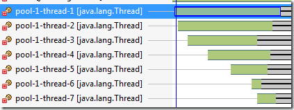
Nice visual of thread pool execution:

Note the lag between the creation of thread pools versus execution times:

Busy

I still wasn’t happy with the serial code being faster than the threaded code.  However, no I knew from looking at the profiled code that threading overhead was significant for the “toy” problem.  So, I thought, what if the methods took longer to run?  In a prior exploration with C# Task parallel computing I had created a “busy” method.  To accomplish the same sort of effect I added in a Thread.sleep(1) to the VehicleLocationCollection::update().  That's a sleep 1ms in an often used method.

Here's the result:

 

Simulation runs: 5 Simulated run time: 60

Serial time: 4.811 Serial time: 4.818 Serial time: 4.818 Serial time: 4.796 Serial time: 4.807

Threaded time: 2.625 Threaded time: 2.518 Threaded time: 2.523 Threaded time: 2.49 Threaded time: 2.509

 

Simulation runs: 5 Simulated run time: 600

Serial time: 58.564 Serial time: 59.062 Serial time: 58.865 Serial time: 59.021 Serial time: 59.399

Threaded time: 30.445 Threaded time: 30.108 Threaded time: 30.084 Threaded time: 31.013 Threaded time: 37.486

I'm glad I thought to make one of the more often used methods more intensive.  To me, this shows that there is indeed an improvement over the serial version when the application crosses a threshold of compute intensity/time versus threading overhead.

Summary

When comparing serial versus parallel code they should both be optimized.  I started with a working serial implementation and transformed it into a threaded version.  Both versions inherit from a common base class.  Unit tests help verify expected behavior.  When transforming to threaded code I found myself using a top down approach.  Methods which iterate over a collection are an easy target for extracting the interior loop body into a method to run as a task.  Transformation of related data structures to thread safe data types is essential.  Try to minimize or eliminate the need for locking/synchronized code.  Too much locking and you just created threaded code which runs in a sequential manner at best.

The TPTP project profiling tool is very useful for profiling threaded applications.  You can quickly identify code that is deadlocked, blocked or waiting.  Your efforts can then be focused appropriately.

Threading is only beneficial once you have enough work to pay the overhead penalty.  Sometimes you are better off using the serial implementation.  ForkJoinTasks take that approach, they fork the problem until it is small enough to process efficiently in a serial way.  The Executors class gives the developer a lot of flexibility in fine tuning the type of thread pool: unlimited, fixed or single.

Good luck in your threading endeavors!

UPCRC Multi-core programming school @ UIUC

One line summary: The UPCRC multi-core programming school was very intense in a good way.

The Material

We eased into things with a basic intro to parallel computing Monday afternoon. Tuesday-Thursday were all very fast paced. We had lecture from 0845-Noon and then again from 1PM to 2PM. At 2PM they would do an overview and introduction of practical labs that corresponded to the days lecture materials.

There were always more labs to choose from than you could complete in a day. So, it was up to the student to pick the labs which they thought would be most beneficial to them. We had lab time between 2:30PM and 5:30PM. During this lab time the lecturers from the day were available. We had a forced :) supper break from 5:30PM-6:15PM. The lab and lecture area were locked up during this time. The lab reopened at 6:15PM and closed at 10:00PM. During this time frame knowledgeable GTA/GRAs were available to answer questions.

I was already somewhat familiar with Java explicit threading so there weren't any surprises there.

OpenMP was probably the easiest to work with and use. It uses pragmas with C++. Visual Studio 2010 has out of the box support for OpenMP.

Intel TBB took some work, but it is more powerful/flexible than OpenMP.

.Net Parallel LINQ (PLINQ) and the Task Parallel Library (TPL) were interesting. It was interesting to work to apply lessons from here in a previous .Net project that does everything in a serial way. It reminded me that we need to make special considerations when ordering is important. Also, you really need to know and understand lambda expressions.

The OpenCL material was by far the hardest. It was difficult in terms of the steps to set up the code and in debugging/figuring out what was going wrong. I was able to complete a Matrix Multiply lab. However, it took about 5 hours. From what I gather only one or two other people completed that lab.

We had a two hour lecture on Thursday regarding vectorizing code. It was very intense and very interesting. I feel like the professor probably covered two weeks of graduate material in those two hours! It was helpful to learn about dependences and how loops could be unrolled or how loops could be changed to allow the compiler to do more optimizing. I need to review the slides and notes from this lecture.  As I recall we covered 48 slides in each of the one hour sessions.

My overall impression is that it is much easier to work with multi-core CPUs than GPUs. The other I noted that there seems to be more focus/maturity in C/C++ support. I'm sure that will change as the SDKs mature.

We wrapped up Friday with a look at an Intel analysis tool and overview of what had been covered and what had not been covered.

Blue Waters

Friday before lunch we toured the future home of the IBM Blue Waters/NCSA facility. It is simply huge. They had what appeared to be many servers in place, but they were actually the power distribution centers! The first floor of the building is all mechanical infrastructure. The building is also set up to be secure facility with swipe cards, PIN entry, retinal scanning and even a "bell" that you are locked in and weighed in.

Summer School Environment

The building facilities, labs, lecture room (power on top of the table at all spots), meals and snacks were all excellent.  The building architecture itself was interesting.  There were many areas inside and outside of the building where you could sit and work.  They also had areas on every floor with seating and whiteboards.

People

Instructors were enthusiastic about the material and were open to questions. It was great that they helped in the labs and were available for questions that were related to the material yet unrelated to the labs. If you had a question about how something they covered might relate to your research they were interested in talking with you and discussing it.

Assistants were knowledgeable and helpful with the lab environment and the labs too.

Staff kept everything running smooth and on time.  They also managed to arrange for good meals and snacks.

The school was also an awesome opportunity to talk with other students from around the world that are interested in this aspect of programming. It was neat to hear the varied application areas that were being considered.

Summary

Overall, a great experience.

http://www.upcrc.illinois.edu/summer/2010/program.html

Something I may consider for next year is another school that they offer:

http://www.vscse.org/summerschool/2010/manycore.html

Data Parallel Computing

Data Decomposition Parallel computing works by using a shared data object with multiple “processors” working on it.

the toy problem

To learn more about Data Decomposition type parallel computing I created a toy application. This entailed creating a demo application that utilized a basic stopwatch instrument, a serial computing class and a parallel computing class.  The application will perform row or column based operations on an 8K by 8K array.

Since I needed to time runs I created a basic stopwatch class. This class provides for starting the stop watch, checking elapsed time and stopping it.

the serial code

I created a serial computing class that initializes an 8K by 8K array of integers and has methods for computing across rows and computing down columns. I created these two methods so that I could see potential differences in working with the array via row or column.

The serial class is used as the baseline which the parallel class is compared against.

I wanted to make sure that the results from the serial and parallel calculations were the same. Therefore, I added methods to the serial class that can be used to check that the parallel results match.

the parallel code

Because the implementation language was Java, the parallel code class extends the Thread class. The Thread class works by using a run() method that takes no arguments. To cope with this, I use a private constructor to determine which method to run. The parallel methods create a new instance which takes arguments for if the row or column method should be called and the start and end value of the domain. These arguments set internal variables which are then used within the run() method.

Psuedo-code for the parallel computation:

computeRowsDomainLimited(int startRow, int endRow)

{

Partsize = size / # threads

Remainder = size % # threads

 

For o = 0 to < # threads

{

Start = o * size

End = start + partSize

computeRowsDomain(start,end)

}

computeRowsDomain(end, end+remainder)

 

Set up threads with the above

Then run them

Then join/wait for all to finish

}

Results

The development machine was a powered by an Intel I7-720 with 6Gig of RAM.  The baseline serial methods and the parallel methods of varying partition/thread size were each run 10 times.  The best run time is used in the calculations.

The code seems to scale well and perform well for the row based computation up to 8 processing threads. Then it seems to drop off a bit and then gradually taper off in performance. I think this corresponds to the machine having 8 logical cores. After 8 the overhead of the additional threads is greater than any potential benefit.

However, the performance the columns seems to peak out around 4 or 5 threads. This could be because of the CPU having 4 real cores with Hyper-Threading. Or it may be that the overhead of accessing non-continuous memory is the determining factor.

Source Code

Source code for the demo application that utilizes the stopwatch class and both the serial and parallel computing classes can be found here:

http://www.dbBear.com/DataDecomposition.zip

In the future I will implement the same computations using OpenCL.

Task Parallel Computing

There are two primary parallel computing techniques: task parallel and data parallel.  Some key aspects to consider if tasks can be run in parallel:

• Are there dependencies between tasks?
• Does the result of the operations change if you change the execution order?
• Will there be contention for data or some other resource?
• Will we get a return on investment for the overhead of configuring and running in parallel?
• Do we have a significant number of tasks to run?  We should have more tasks to run than we have cores.

Batch processing

I created a BatchProcessor solution with a console application called BPRun.  This project runs a setup portion, the parallel tasks and then the teardown jobs.   The tasks to run are specified in corresponding configuration files.  I use code similar to this in production for batch processing ~20 DOS .bat jobs.  Being able to have jobs run in a parallel fashion has resulted in a significant time savings.

Setup and Teardown

The setup and teardown portions of the application are run in a serial fashion.  The items in the configuration files are executed one after another.  Comments may be placed in the file with // prefixing.

Task Parallel

The task parallel section executes the items in the corresponding configuration file.  As a task finishes the scheduler picks up and runs the next job on that process.  The code that does this is in a corresponding Processor class.

Tasks with dependencies

What if you have a task that has a dependency?  You can chain them.  That is, have the first process or task call the second or dependent task upon completion.  For instance, you may have a job that does some data prep and then chain it to call a task that does analysis.

Keeping Busy

On *nix systems we have the sleep command which we can use to pause for the given # of seconds.  However, this doesn’t place any load on the machine.  I wanted the machine to have a load placed on it by the tasks so that we could see that it is really taxing the machine.  To that end I created a small console application called Busy.  This takes the number of seconds to be busy as a parameter.

Download

You can get the source code for the Batch Processor and the Busy application here: https://github.com/k0emt/BatchProcessor

Video

See a video tour of the code for Busy and the Batch Processor along with demos of the applications here:

Selecting a machine for OpenCL / GPGPU use

What is GPGPU computing?  GPGPU stands for General Purpose computing on Graphics Processor Units.  The basic idea is that we use the graphics card to do some computing.  Today most computers have 2 cores and some as many as 6.  With hyper-threading we may see what appears to be double that many processors.  However, a video card such as the NVidia 480 has “cores” or processors.

Portable or Desktop?

If you choose a portable machine you will be able to take the unit with you for presentations, research or on the go development.  However, you will typically sacrifice in the power or number of cores that the video card has available.  For instance a laptop with a GT330M has 48 cores.  A desktop with a GT330 has 96-112 cores.

You’ll also likely have a much harder time finding a suitable laptop.  When choosing a desktop, go for a mini-tower case or one that can be purchased with the appropriate video card.  Current video cards often take additional power from the power supply and require additional ventilation.  For instance, you could purchase an HP HPE-380T with an NVidia GTX260 with 1.8G of DDR3 RAM and 192 cores!

ATI or NVidia?

NVidia is known for its CUDA entry.  ATI has ATI Stream computing.  Both companies now have drivers for OpenCL.  I chose to go with NVidia because I was able to find my resources for their products.  ATI Stream is fairly new.

Whichever you choose, you will need to know what type of computing/gaming you plan to do and if there is existing support for that.  Also, you will need to make sure to check the manufacturers pages to see if the video card you have selected is supported for GPGPU use.

Cores, speed

In general, the more cores or shaders the better.  Also pay attention to how fast they are running.

Memory

What type of memory? In general you want to stay away from shared memory.  This makes use of the slower system memory and steals resources from the PC.  Look for DDR3 or DDR5 memory.  Sometimes they are prefixed with a G like GDDR3.  In general DDR5 is faster.

How much memory?  After consulting with a professor with experience in the field he suggested 512M minimum.  If you can get more that is preferred. 

Sony CW, F and Z series

Because I wanted to be portable and have the minimum 512M with an NVidia card, I considered the Sony CW, F and Z series computers.

However, these machines are new enough that the released video drivers do NOT support OpenCL.  I did find that there is a way to modify the released NVidia drivers to work on them.

http://forum.notebookreview.com/sony/472664-vaio-f-nvidia-drivers-update-197-16-gt-330m-10de-0a29.html

After using the information above, I was able to run the Particles demo from here:

http://code.google.com/p/nativelibs4java/wiki/OpenCL

However, the hardware identification and mandelbrot set generator on that site don't work.

I also downloaded and tested a CUDA based mandelbrot application that was listed on the NVidia featured applications site.  It ran nicely.